How Positional Encoding Evolved in Transformers: From Sinusoidal Encoding to RoPE

I’m going to explain how the way we incorporate positional information when calculating attention has evolved: from the original fixed positional encoding, to relative positional encoding, and finally to RoPE (Rotary Positional Encoding).

original

We can define the process of calculating attention in the transformer as follows

1. Obtain Q, K, and V by incorporating word embeddings, positional information, and the $W_{q,k,v}$ matrices. In the paper, they encapsulate step 1 as the function $f_{q,k,v}$.

$$q_m = f_q(x_m, m)$$ $$k_n = f_k(x_n, n)$$ $$v_n = f_v(x_n, n)$$

Here in $f_{q,k,v}$, we add sinusoidal positional information to the word embeddings and then perform matrix multiplication with $W_{q,k,v}$.

$$f_{t:t\in\{q,k,v\}}(x_i,i) := W_{t:t\in\{q,k,v\}}(x_i+p_i)$$

where each positional encoding is defined as follows:

$$\begin{cases} p_{i,2t} = \sin\left(k/10000^{2t/d}\right) \\ p_{i,2t+1} = \cos\left(k/10000^{2t/d}\right) \end{cases}$$

2. With the obtained Q, K, and V, calculate the attention scores as follows.

$$a_{m,n} = \frac{ \exp\left(\frac{q_m^T k_n}{\sqrt{d}}\right) }{ \sum_{j=1}^{N} \exp\left(\frac{q_m^T k_j}{\sqrt{d}}\right) }$$ $$o_m = \sum_{n=1}^{N} a_{m,n}v_n$$

Since $q_m$ is $W_q(x_m + p_m)$ and $k_n$ is $W_k(x_n + p_n)$, the ‘$q_m$ transposed @ $k_n$’ can be written as follows:

$$q_m^T k_n = x_m^T W_q^T W_k x_n + x_m^T W_q^T W_k p_n + p_m^T W_q^T W_k x_n + p_m^T W_q^T W_k p_n$$

relative -1

The authors of Self-Attention with Relative Position Representations (Shaw et al., 2018) came up with relative positional encoding, which measure the relative positional encoding. The main idea of relative pos encoding is this:

At that time, fixed positional encoding had a problem: regardless of context, we were training the transformer to treat position $n$ as having the same meaning all the time. Because of this, the model couldn’t easily generalize to longer sequences than those seen during training, since absolute positions beyond the training range were not encoded (whereas with relative encoding, it can!).

To handle this issue, they came up with relative positional encoding, which provides positional information by letting the transformer know how far apart two tokens are, rather than relying on their raw positions. This significantly improved the performance of LLMs and made it possible to generalize beyond the training range.

Here is more details on how they applied relative pos encoding.

• replaced $p_m$ in third and fourth term into a trainable vector $u^T$ and $v^T$.
  => To make the attention score independent of the query’s specific location. using two different learnable vectors $u$, $v$ allows the model to learn two distinct types of positional bias

• replaced $p_n$ in second and fourth term into $p_{m-n}$. => Because we wanted to apply relative position to the key

• and replaced $W$ into tilda $W$ where its get matrix multiplied with positional embeddings => $W_k$ becomes an expert at processing content, $\tilde{W}_k$ becomes an expert at processing relative positions.

these changes resulted in

$$q_m^T k_n = x_m^T W_q^T W_k x_n + x_m^T W_q^T \tilde{W}_k \tilde{p}_{m-n} + u^T W_q^T W_k x_n + v^T W_q^T \tilde{W}_k \tilde{p}_{m-n}$$

You can also understand in this way:

$$x_m^T W_q^T W_k x_n$$

This is content-to-content attention.

It measures attention between the content at position $m$ and the content at position $n$.

There is no positional information here, so nothing needs to change.

$$x_m^T W_q^T W_k p_n$$

This is query-content to key-position attention.

Originally, it uses the key’s absolute position $p_n$.

For relative position, we want the key position relative to the query:

$$p_n \rightarrow p_{m-n}$$

So now the attention depends on the distance between the query and key.

$$p_m^T W_q^T W_k x_n$$

This is query-position to key-content attention.

The problem is that $p_m$ is the query’s absolute position.

If we keep $p_m$, the attention score still depends on whether the query is at position 5, 20, 100, etc.

So we remove that absolute-position dependence:

$$p_m \rightarrow u$$

where $u$ is a learned vector shared across positions.

Now this term represents a global attention bias toward key content, independent of the query’s absolute position.

$$p_m^T W_q^T W_k p_n$$

This is query-position to key-position attention.

We want this to depend only on relative position.

So:

$$p_n \rightarrow p_{m-n}$$

and:

$$p_m \rightarrow v$$

This gives:

$$v^T W_q^T \tilde{W}_k p_{m-n}$$

So this term now represents attention bias based on relative distance $m-n$, independent of the query’s absolute position.

The main idea is simply:

$$\boxed{p_n \rightarrow p_{m-n}}$$

to make the key position relative to the query,

and

$$\boxed{p_m \rightarrow u,v}$$

to remove the query’s absolute position from the attention score.

relative -2

Later, prople found that the last three terms in relative-1 didn’t contribute much when calculating attention, so researchers replace those three blocks with $b_{i,j}$.

$$q_m^T k_n = x_m^T W_q^T W_k x_n + b_{i,j}$$

relative -3

Authors of the T5 paper found out that second and third term in the original actually don’t contribute much when calculating the attention, so they simply replaced thosr terms with $b_{i,j}$, and replaced the fourth term $pWWp$ with $pUUp$.

why replaec W with U?

Because Ws are Content Matrices. Their entire purpose is to learn the best way to project the token’s content or meaning ($x_m$ and $x_n$) into the query and key spaces. They are optimized to work with semantic information. So they introduced new matrices U which wil be optimized for projecting positional information.

$$q_m^T k_n = x_m^T W_q^T W_k x_n + p_m^T U_q^T U_k p_n + b_{i,j}$$

relative -4

In the original term, replace the all fixed positional encoding with relative positional encoding and then dropped the last term(position-position).

$$q_m^T k_n = x_m^T W_q^T W_k x_n + x_m^T W_q^T W_k \tilde{p}_{m-n} + \tilde{p}_{m-n}^T W_q^T W_k x_n$$

RoPE

<background of RoPE>

To improve positional encoding, instead of adding positional information, RoPE rotates the word embedding multiplied with W matrices($W_qx_m$ and $W_kx_n$) So that dot product between two adjacent word embeddings will get higher score and vice versa.

$$f_q(x_m,m) = (W_qx_m)e^{im\theta}$$ $$f_k(x_n,n) = (W_kx_n)e^{in\theta}$$

For simplicity, let’s assume the embedding dimension is just 2, so the word embedding for a token is $(x_1,x_2)$. To mathematically describe rotation, we can treat this 2D vector as a complex number.

Btw Rotating a complex vector can indeed be expressed like this

$$f_{\{q,k\}}(x_m,m) = \begin{pmatrix} \cos m\theta & -\sin m\theta \\ \sin m\theta & \cos m\theta \end{pmatrix} \begin{pmatrix} W_{\{q,k\}}^{(11)} & W_{\{q,k\}}^{(12)} \\ W_{\{q,k\}}^{(21)} & W_{\{q,k\}}^{(22)} \end{pmatrix} \begin{pmatrix} x_m^{(1)} \\ x_m^{(2)} \end{pmatrix}$$

Then, to compute the attention, we take the dot product between two rotated embeddings ($f_q$ and $f_k$). Since the dot product between two complex vector $u$ and $v$ is $uv^*$, we do multiplication of $f_q$ and $f_k^*$)

$$g(x_m,x_n,m-n) = \operatorname{Re} \left[ (W_qx_m)(W_kx_n)^*e^{i(m-n)\theta} \right]$$

Now let’s scale this up: when the embedding dimension is larger than 2, we split the embedding into $d_{\text{model}}/2$ blocks. Each block is treated as a 2D vector and rotated separately. So for the full embedding, the rotation can be expressed like this:

$$f_{\{q,k\}}(x_m,m) = R_{\Theta,m}^{d} W_{\{q,k\}}x_m$$

where

$$R_{\Theta,m}^{d} = \begin{pmatrix} \cos m\theta_1 & -\sin m\theta_1 & 0 & 0 & \cdots & 0 & 0 \\ \sin m\theta_1 & \cos m\theta_1 & 0 & 0 & \cdots & 0 & 0 \\ 0 & 0 & \cos m\theta_2 & -\sin m\theta_2 & \cdots & 0 & 0 \\ 0 & 0 & \sin m\theta_2 & \cos m\theta_2 & \cdots & 0 & 0 \\ \vdots & \vdots & \vdots & \vdots & \ddots & \vdots & \vdots \\ 0 & 0 & 0 & 0 & \cdots & \cos m\theta_{d/2} & -\sin m\theta_{d/2} \\ 0 & 0 & 0 & 0 & \cdots & \sin m\theta_{d/2} & \cos m\theta_{d/2} \end{pmatrix}$$

And for computational efficiency, it can be simplified as follows:

$$R_{\Theta,m}^{d}x = \begin{pmatrix} x_1 \\ x_2 \\ x_3 \\ x_4 \\ \vdots \\ x_{d-1} \\ x_d \end{pmatrix} \otimes \begin{pmatrix} \cos m\theta_1 \\ \cos m\theta_1 \\ \cos m\theta_2 \\ \cos m\theta_2 \\ \vdots \\ \cos m\theta_{d/2} \\ \cos m\theta_{d/2} \end{pmatrix} + \begin{pmatrix} -x_2 \\ x_1 \\ -x_4 \\ x_3 \\ \vdots \\ -x_d \\ x_{d-1} \end{pmatrix} \otimes \begin{pmatrix} \sin m\theta_1 \\ \sin m\theta_1 \\ \sin m\theta_2 \\ \sin m\theta_2 \\ \vdots \\ \sin m\theta_{d/2} \\ \sin m\theta_{d/2} \end{pmatrix}$$

Quick Final Summary of RoPE

In the RoPE(Rotatry Positional Encoding), we rotate word embeddings in following ways:

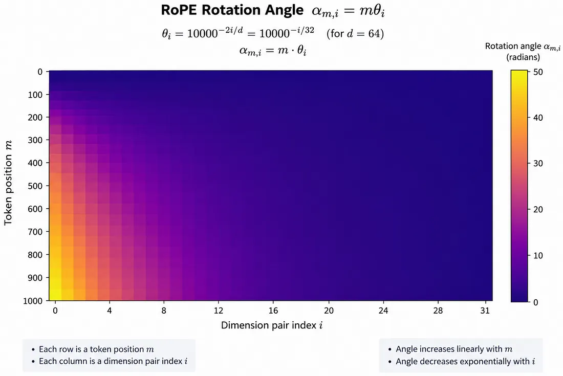
Divied each token’s word embeddings into emedding_dim / 2 number of pairs(each pair just two blocks). Then we rotate each of these pairs by

$$\alpha_{m,i} = m\theta_i$$

where $\theta_i$ is defined as

$$\theta_i = 10000^{-2i/d}$$

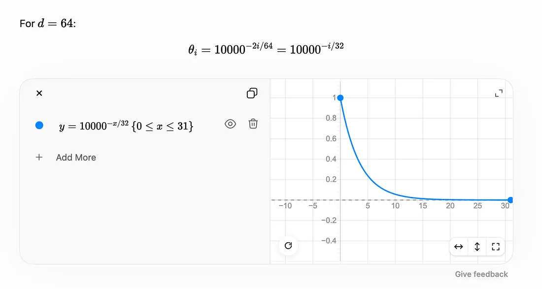
The value of $\theta_i$, degrades fast as $i$ increases, as a result fornt part of word embeddings got rotated faster(high frequency) and rear part of word embeddings get rotated much slower(low frequency)? So Why did they designed RoPE in this way?

Front Part (High Frequencies) = Millimeter Markings

• The first few pairs of dimensions rotate very fast. A change in position from $m=5$ to $m=6$ causes a large change in their rotation. This is crucial for understanding local grammar, syntax, and phrasing (e.g., “New York” vs. “York New”).

Rear Part (Low Frequencies) = Meter & Kilometer Markings

• The dimensions toward the end rotate very, very slowly. A change in position from $m=5$ to $m=6$ causes almost no change in their rotation. It takes a large jump, like from $m=5$ to $m=105$, to see a meaningful angular change.