4 Types of Normalization

There are four main types of normalization commonly used in ML. This post explains each type of normalization, when it is used, and generally why normalization is used in ML. Anyway, this post covers Batch Norm, Layer Norm, Instance Norm, and Group Norm.

Batch Norm

When the input is ((N, H, W, C)), normalization is performed on each ((N, H, W)). So in total, (C) separate normalization operations happen. It is usually used in CNNs. For reference, look at the image below.

Why Do Batch Norm in CNN?

In a CNN, each channel represents a different learned feature map. For example, one channel may respond strongly to edges, while another may respond to textures or other visual patterns. Because each channel can have a different activation distribution, BatchNorm is a suitable choice since it normalizes each channel separately.

Layer Norm

Layer Norm is usually applied to the outputs of Transformer sublayers such as MHA. When the tensor shape is ((N, L, D)), normalization is performed over each (D)-dimensional vector, so in total, (N \times L) separate normalization operations happen.

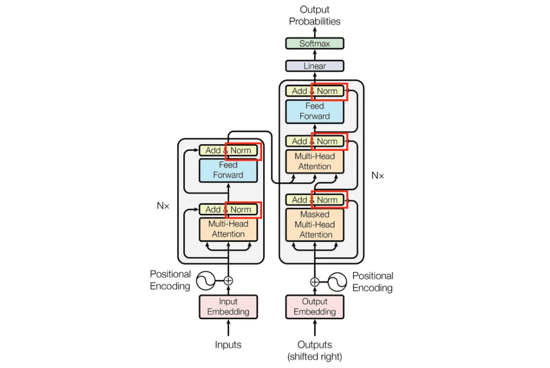
Why do LayerNorm in transformer?

LayerNorm is used in Transformers to keep each token’s hidden representation at a stable scale as it passes through attention and feed-forward layers. For every token independently, it normalizes that token’s values across the hidden dimension (D). This avoids dependence on batch size or other token positions, makes training more stable, and helps prevent activations from becoming excessively large or small as the network gets deeper.

Instance Norm

If the tensor shape is (N, H, W, C), it happens to (H, W) So intotal N*C times of normalization happening here. Instance Norm usually happens to Style Transfer

Quick Review of the Style Transfer

Style Transfer is a technique that combines a content of one image(ex, a San Francisco ity view) and style of another image(ex, The starry Night by Vincent can Gogh, 1889)

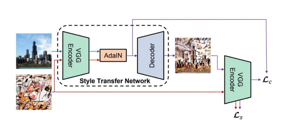
The process begins with a content image and a style image, which are both passed through a pre-trained VGG Encoder to extract the structural features of the content and the textural and color features of the style. These encoded features are then fed into the AdaIN (Adaptive Instance Normalization) block, which aligns the mean and variance of the content features to match those of the style features, effectively blending the style onto the content’s structure in the feature space. Finally, these modified features are passed through a Decoder that translates them back into a standard pixel image, producing the final stylized output.

The process begins with a content image and a style image, which are both passed through a pre-trained VGG encoder to extract the structural features of the content and the textural and color features of the style. These encoded features are then fed into the AdaIN (Adaptive Instance Normalization) block, which aligns the mean and variance of the content features to match those of the style features, effectively blending the style onto the content’s structure in feature space.

Finally, these modified features are passed through a decoder that translates them back into a standard pixel image, producing the final stylized output.

Why use AdaIn in Style Transfer?

AdaIN is used because, in feature space, the per-channel mean and variance carry a lot of the image’s style information, while the spatial pattern inside each feature map carries more of the content structure.

Suppose the encoded content and style features have shape

$$(H, W, C)$$

For each channel (c), AdaIN looks at the corresponding (H \times W) feature map.

Why normalize each (H \times W)?

Each channel is a separate learned feature map. For example, one channel may respond to a certain texture, another to edges, another to colors, and so on.

For the content feature (x), AdaIN computes

$$\frac{x-\mu(x)}{\sigma(x)}$$

where (\mu(x)) and (\sigma(x)) are calculated over (H \times W), separately for each channel.

This removes that channel's original mean and variance while keeping its spatial pattern.

So roughly:

• spatial arrangement in (H \times W) → content structure
• per-channel mean and variance → style-related statistics

That is why normalization is performed over (H \times W), independently for every channel.

Why normalize only the content?

Because the goal is:

remove the content's style statistics and replace them with the style image's statistics.

First, the content statistics are removed:

$$\hat{x} = \frac{x-\mu(x)}{\sigma(x)}$$

Then the style image's statistics are injected:

$$\sigma(y)\hat{x}+\mu(y)$$

So the complete operation is

$$\mathrm{AdaIN}(x,y) = \sigma(y) \left( \frac{x-\mu(x)}{\sigma(x)} \right) + \mu(y)$$

where:

• (x) = content features
• (y) = style features

The style features are not normalized because their mean and variance are exactly the information we want to transfer.

If we normalized the style features too and then discarded their original mean and variance, we would remove the style information that AdaIN is trying to copy.

So the intuition is simply:

$$\text{Content} \xrightarrow{\text{remove its }\mu,\sigma} \text{Normalized Content} \xrightarrow{\text{apply style }\mu,\sigma} \text{Stylized Content}$$

Group Norm

In group norm, split the channles into G Groups, and then normalize per groups, so normlaization is happening to each (C/G, H, W) and total G*N times of normalization happens. It usually happens in Masked R-CNN

Quick Review of Masked R-CNN

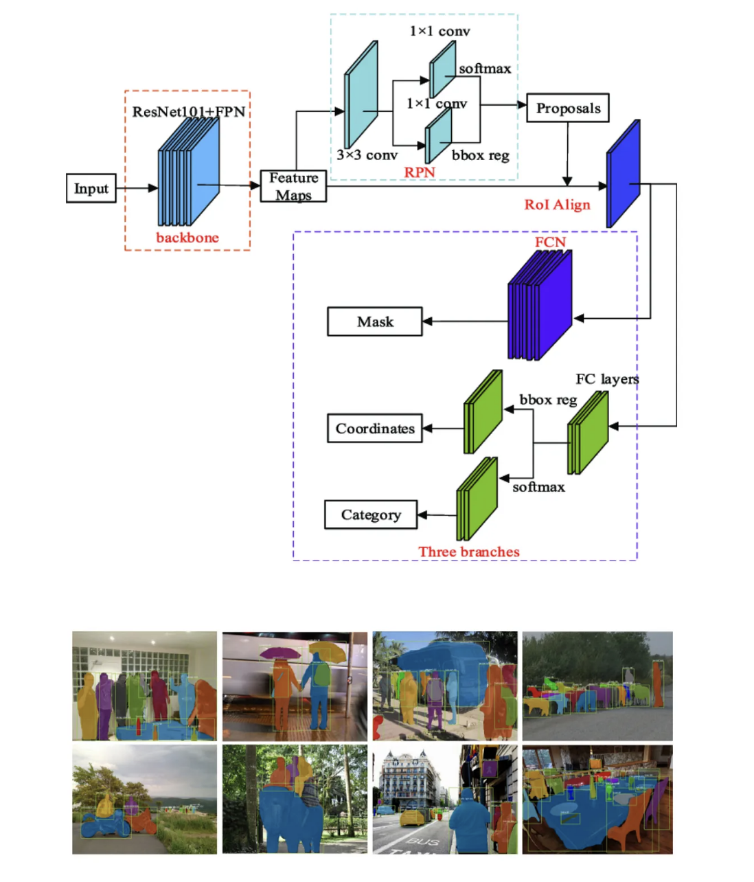
Ideally, we would want to use Batch Normalization (BN) so the model can learn common features across a diverse set of images. However, since we are handling high-resolution images in object detection, memory bottlenecks force us to drop the batch size down to something as small as N=2. At this size, we are no longer getting a stable, universal average of the dataset. Instead, we just get the erratic, wildly swinging average of two random images, which completely destabilizes training. That is where Group Normalization (GN) has to take over.

Before jumping to GN, we might think about using Instance Normalization (IN). However, IN is designed to capture specific stylistic details by normalizing every single channel independently. For example, if we have 32 channels detecting a car wheel, IN squashes the “metallic rim” channel and the “dark rubber” channel flat on their own.

Imagine the “metallic rim” channel is naturally very bright (high activation) because metal is shiny. The “dark rubber” channel is naturally very dim (low activation) because tires are black. The neural network recognizes a “wheel” specifically by seeing this exact contrast: a bright circle surrounded by a dark circle. If you apply Instance Normalization, it forces every individual channel to have the exact same average brightness.

It takes the bright rim channel and forcefully dims it down to average. It takes the dark rubber channel and forcefully brightens it up to average. Now, both channels have the exact same flat intensity. The contrast between them is completely erased. Because that bright-to-dark relationship is destroyed, the network loses the structural context it needs to recognize the object as a wheel.

This destroys the relative differences in activation strength between those channels, wiping out the combined information the network needs to recognize the wheel.

GN solves this by taking those G related channels, putting them into one group, and calculating a single mean and variance for that entire group. By scaling the whole group together, GN preserves the relative differences between the channels. If the “metallic rim” channel is firing twice as hard as the “rubber” channel, GN scales them both simultaneously, keeping that crucial 2:1 ratio intact.