Llama 2

Meta first pretrained the Llama 2 base model, then fine-tuned it on about 27,500 high-quality instruction–response examples to create the initial Llama 2-Chat model. They then iteratively improved this chat model through repeated SFT and RLHF stages, producing Llama 2-Chat V1 through V5.

Build Llama 2-Chat V1 to V5

Procedure 1: V1–V3

• Performed SFT using datasets created through rejection sampling.
• At each version, generated multiple responses, selected the best responses, and used them for the next round of SFT.

Procedure 2: After V3

• Performed additional SFT using Ghost Attention data.

Procedure 3: V4

• Performed SFT using rejection-sampling data.
• Used good responses collected from V1, V2, and V3, instead of using only the latest version.

Procedure 4: V5

• Performed another round of SFT using rejection-sampling data, including good responses from previous versions.
• Then applied PPO training.

How the SFT Training Data Was Built

At each RLHF iteration (V1→V5), Meta needed fresh, high-quality training data to fine-tune the model. They didn’t just use one method — they built a composite dataset from four different sources, each targeting a different goal.

Source 1: Helpfulness Data (Rejection Sampling)

For a given prompt, they sample (K) different responses from the current model. Then they score all (K) responses using the helpfulness reward model and keep only the single best one. This best (prompt, response) pair becomes a new training example.

Source 2: Safety Data — Easy Cases (Rejection Sampling)

Same idea as helpfulness, sample (K) responses to an adversarial prompt, score them with the safety reward model, and keep the safest one.

Source 3: Safety Data — Hard Cases (Context Distillation)

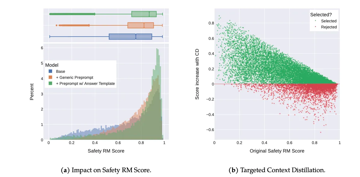
This uses a clever trick called context distillation. They prepend a safety instruction (e.g., “You are a safe and responsible assistant”) to the adversarial prompt, which nudges the model into generating a safer response. Then they train the model on this safer response without the safety preprompt.

They generate two responses — one with the safety preprompt and one without — and use the safety reward model to decide which is better. They only keep the context-distilled version if it actually scores higher.

Why not use context distillation for everything? As shown in Figure 16b of the paper, when the model’s original response was already safe and high-quality, context distillation often made it worse. The preprompt caused the model to give overly cautious, generic, “preachy” responses that scored lower than the original. So they only applied it selectively — on the hard cases where the original response was poor.

Source 4: Human-Written Safety Responses

A dedicated red team actively tried to break/jailbreak the model. When they found prompts that consistently bypassed safety guardrails, human annotators manually wrote ideal safe responses for those specific prompts. These hand-crafted examples were added directly to the training set.

Additional Details

The following sections take a closer look at several techniques and implementation details introduced in the paper.

Ghost Attention

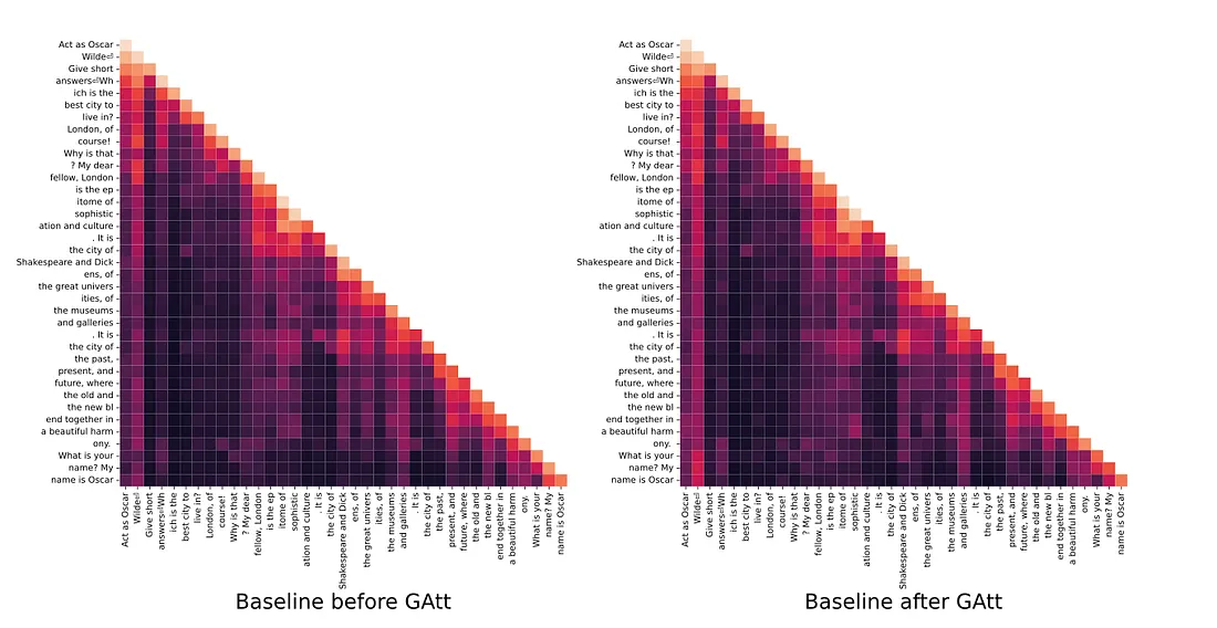
LLMs tend to forget the initial system instruction over the course of a multi-turn conversation. For example, even if the model is told to “Act as Elon Musk” at the start, it gradually loses track of that instruction after several turns. To address this, the authors introduced Ghost Attention (GAtt).

How it works:

1. Inject the instruction into every user turn. The system instruction (e.g., “Act as Elon Musk”) is concatenated to each user message throughout the conversation, not just the first one.

2. Generate responses using this augmented data. Because the model now sees the instruction at every turn, its responses consistently stay in character.

3. Fine-tune using the generated response, but remove the repeated instructions from later turns. To avoid a mismatch caused by those earlier generated turns, set the loss to zero for all previous-turn tokens and train only on the final assistant response.

Generation:

Instruction + User 1 → Assistant 1
Instruction + User 2 → Assistant 2
Instruction + User 3 → Assistant 3

Training:

Instruction + User 1 → Assistant 1
User 2 → Assistant 2
User 3 → Assistant 3 ← loss only here

In the paper’s attention visualizations (Figure 10), the column corresponding to the system instruction is noticeably brighter after GAtt training, confirming that the model pays stronger attention to the initial instruction across all turns.

The PPO Equation Used During V4 and V5

$$\arg\max_{\pi} \mathbb{E}_{p \sim \mathcal{D},\, g \sim \pi} \left[ R(g \mid p) \right]$$ $$R(g \mid p) = \tilde{R}_c(g \mid p) - \beta D_{KL} \left( \pi_\theta(g \mid p) \parallel \pi_0(g \mid p) \right)$$

More details on each term:

1. $R_c$ Term

$$R_c(g \mid p) = \begin{cases} R_s(g \mid p), & \text{if } \mathrm{IS\_SAFETY}(p) \text{ or } R_s(g \mid p) < 0.15 \\ R_h(g \mid p), & \text{otherwise} \end{cases}$$ $$\tilde{R}_c(g \mid p) = \mathrm{WHITEN} \left( \mathrm{LOGIT} \left( R_c(g \mid p) \right) \right)$$

2. $\beta$ Term

KL divergence penalty term that prevents the model’s distribution from changing too much from the original SFT model.

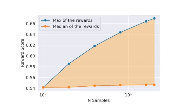
Why use rejection sampling?

As you can see in the diagram below (Figure 7), the quality of a typical or average model response (the median) stays flat, no matter how many samples you generate. However, the quality of the single best response (the max) increases significantly the more samples you generate. So by doig rejection sampling we can select the best of best prompt and response pair and use it again to SFT.