Core Probability Theories

This post outlines the fundamental probability concepts essential for machine learning: Maximum Likelihood Estimation (MLE), Conditional Probability, Marginal Distribution, Bayes’ Theorem, the Central Limit Theorem (CLT), and KL Divergence.

Joint Probability

For any two events (A, B), always:

$$P(A,B) = P(A \mid B)P(B)$$

or equivalently,

$$P(A,B) = P(B \mid A)P(A)$$

If (A) and (B) are independent, then:

$$P(A \mid B) = P(A)$$

so the joint simplifies to:

$$\boxed{P(A,B) = P(A)P(B)}$$

If they are dependent, you cannot simplify it like that:

$$\boxed{P(A,B) = P(A \mid B)P(B)}$$

MLE (Maximum Likelihood Estimation)

Maximum Likelihood Estimation (MLE) is a method for choosing model parameters so that the observed data becomes as “likely” as possible under the model.

For a simple example, refer to the following diagram. Which distribution seems to explain the data points well?

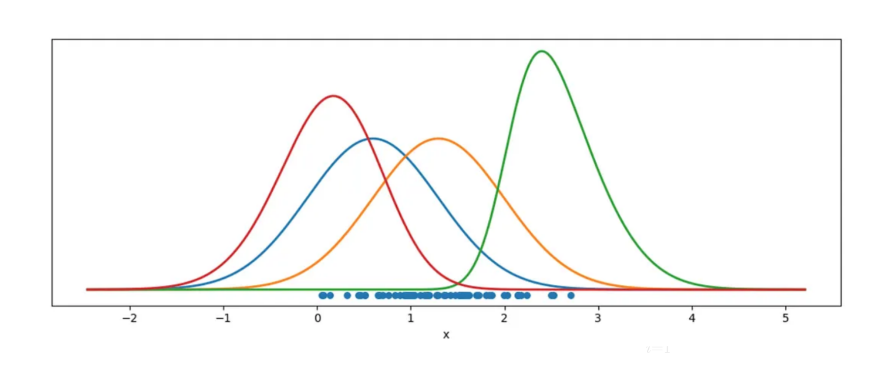
To determine this, we calculate (P(x_1) * P(x_2) * \cdots * P(x_n)) for each distribution to see which one yields the highest value. In this diagram, the third distribution will certainly have the highest value. Here finding distributon equals to finding mean and std, parameters that can maximize the thing.

Here, finding the best distribution is equivalent to finding the mean and standard deviation(which determine shape and position of each distribution) — the parameters that maximize the likelihood.

We can summarize this as finding the theta that maximizes L(theta).

$$L(\theta) = P(x_1 \mid \theta) \cdot P(x_2 \mid \theta) \cdots P(x_n \mid \theta) = \prod_{i=1}^{n} P(x_i \mid \theta)$$

However, since multiplying many probabilities can cause numerical issues, we usually apply a logarithm to turn the product into a summation:

$$\log L(\theta) = \log\left( \prod_{i=1}^{n} P(x_i \mid \theta) \right) = \sum_{i=1}^{n} \log P(x_i \mid \theta)$$

Conditional Probability

Conditional probability is the probability of an event occurring given that another event has already occurred.

$$P(A \mid B) = \frac{P(A \cap B)}{P(B)}, \qquad \text{if } P(B) > 0$$

“the probability of A given B.”

if A and B are independent (P(A,B) = P(A)P(B)) so (P(A \mid B) = P(A)P(B) / P(B))

resulting in (P(A \mid B) = P(A)).

Marginal Distribution

If you have a joint distribution (P(A,B)), the marginal distribution of (A) is obtained by summing over all possible values of (B):

$$P(A) = \sum_b P(A,b)$$

Example:

Suppose a university records whether a student passes an exam and whether they attended review sessions.

$$P(\text{Passed}) = P(\text{Passed}, \text{Attended}) + P(\text{Passed}, \text{Did not attend}) = 0.3$$ $$P(\text{Failed}) = P(\text{Failed}, \text{Attended}) + P(\text{Failed}, \text{Did not attend}) = 0.7$$

Bayes’ Theorem

$$P(A \mid B) = \frac{P(B \mid A)P(A)}{P(B)}$$

• $P(A)$: Prior — belief about A before seeing B
• $P(B \mid A)$: Likelihood — probability of observing B if A is true
• $P(B)$: Evidence — overall probability of observing B
• $P(A \mid B)$: Posterior — updated belief about A after seeing B

Let’s say we want to compute (P(S \mid C_1))— the probability of meeting a single person given that you go to Club 1.

We can calculate this using Bayes’ theorem. For simplicity, assume there are only two clubs in the city: Club 1 and Club 2.

First seeing a Single from a Club 1 can be represented as

$$P(S \mid C_1) = \frac{P(S, C_1)}{P(C_1)}$$

and by extending (P(C_1, S)) it can be re-written as following(which is Bayes Theorem)

$$P(S \mid C_1) = \frac{P(S)P(C_1 \mid S)}{P(C_1)}$$

Now, we can expand the denominator using the law of total probability:

$$P(C_1) = P(C_1, S) + P(C_1, M)$$

So the expression becomes:

$$P(S \mid C_1) = \frac{P(S)P(C_1 \mid S)} {P(C_1,S) + P(C_1,M)}$$

Next, we rewrite the joint probabilities:

$$P(C_1,S) = P(S)P(C_1 \mid S)$$ $$P(C_1,M) = P(M)P(C_1 \mid M)$$

Substituting these back in:

$$P(S \mid C_1) = \frac{P(S)P(C_1 \mid S)} {P(S)P(C_1 \mid S) + P(M)P(C_1 \mid M)}$$

Now everything becomes measurable

• $P(S)$, $P(M)$: We can obtain these from government statistics (for example, the proportion of single and married people in the city).
• $P(C_1 \mid M)$, $P(C_1 \mid S)$: We can estimate these by surveying married and singles asking which club they usually go to.

Once we have those values, we can compute $P(S \mid C_1)$.

Central Limit Theorem

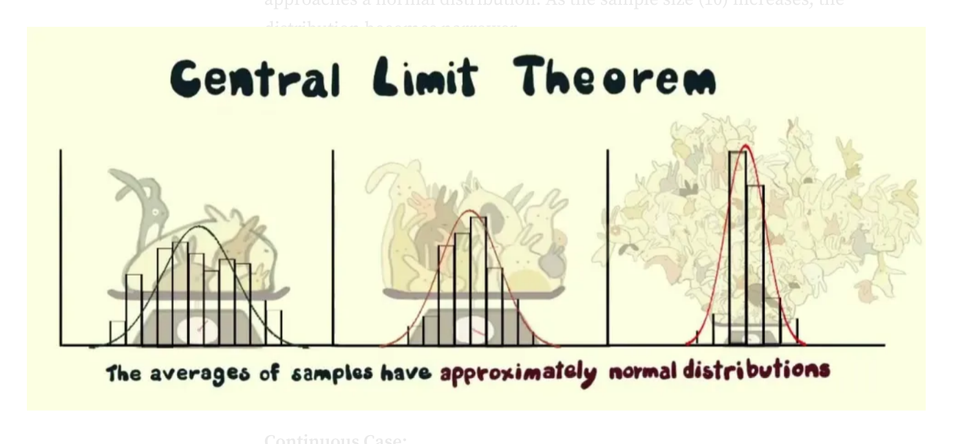
Suppose someone wants to estimate the weight distribution of bunnies in a mountain. In reality, it is not possible to catch all the bunnies. So he repeats the following process:

1. Catch 10 bunnies

2. Compute the average weight and record it

3. Release the bunnies

As he continues this process, the distribution of the recorded averages approaches a normal distribution. As the sample size (10) increases, the distribution becomes narrower.

KL Divergence

KL Divergence can be expressed in two types: the discrete case and the continuous case.

Discrete Case:

$$D_{KL}(P \parallel Q) = \sum_i P(i)\log\frac{P(i)}{Q(i)}$$

Continuous Case:

$$D_{KL}(P \parallel Q) = \int P(x)\log\frac{P(x)}{Q(x)}\,dx$$

=> How different Q looks when P is treated as the reference / true distribution.

Let me first show how the equation for the discrete case can be derived, and then explain the continuous case.

1. Discrete Case

Let’s assume we have two coins, Coin 1 and Coin 2, and we want to measure how Coin 2’s distribution is different from Coin 1.

$$\text{Coin 1} \begin{cases} p_1 & \text{heads} \\ p_2 & \text{tails} \end{cases} \qquad \text{Coin 2} \begin{cases} q_1 & \text{heads} \\ q_2 & \text{tails} \end{cases}$$

To do this, we make an observation by throwing Coin 1 (N) times and recording the number of heads (N_H) and tails (N_T).

Then, we can compare how likely this observation is coming from Coin 1 versus Coin 2 using a likelihood ratio:

$$\frac{P(\text{observation} \mid \text{coin1})} {P(\text{observation} \mid \text{coin2})} = \frac{p_1^{N_H} \cdot p_2^{N_T}} {q_1^{N_H} \cdot q_2^{N_T}}$$

Apply Log and Normalize: To make the numbers manageable, we take the Log and divide by (N) (the total number of throws):

$$\frac{1}{N} \log \left( \frac{p_1^{N_H} \cdot p_2^{N_T}} {q_1^{N_H} \cdot q_2^{N_T}} \right)$$

Expansion: Using log rules, we can break this down:

$$\frac{N_H}{N}\log p_1 + \frac{N_T}{N}\log p_2 - \frac{N_H}{N}\log q_1 - \frac{N_T}{N}\log q_2$$

Final Result (KL Divergence): Here is the key trick: if we throw the coin enough times (as (N \to \infty)), the frequency of heads (N_H/N) becomes the true probability (p_1). (Here (N = N_H + N_T))

So the equation becomes:

$$p_1 \log p_1 + p_2 \log p_2 - p_1 \log q_1 - p_2 \log q_2$$

Which simplifies to:

$$p_1 \log \frac{p_1}{q_1} + p_2 \log \frac{p_2}{q_2}$$

2. The Continuous Case

Now let me explain the continuous case. For this, just think about what happens if we don’t have just two classes (heads/tails), but infinite classes.

When we move to a continuous space, we can’t sum up specific points anymore because the “width” of each point becomes infinitely small.

Mathematically, this just means the Summation ((\Sigma)) transforms into an Integral ((\int)). The logic remains exactly the same, but we are summing the area under the curve instead of discrete blocks.

So the final term becomes:

$$\int p(x)\log\frac{p(x)}{q(x)}\,dx$$

This measures how (Q) is different from (P).